Synthetic temporal network with community structure

This example uses SynthTempNetwork to generate a synthetic continuous-time temporal network of 12 agents organised into three communities of four. Within-community contacts are more frequent than cross-community ones (block probability structure).

The simulation produces a stream of time-stamped contact events that are then loaded into a ContTempNetwork for analysis.

Two plots are produced:

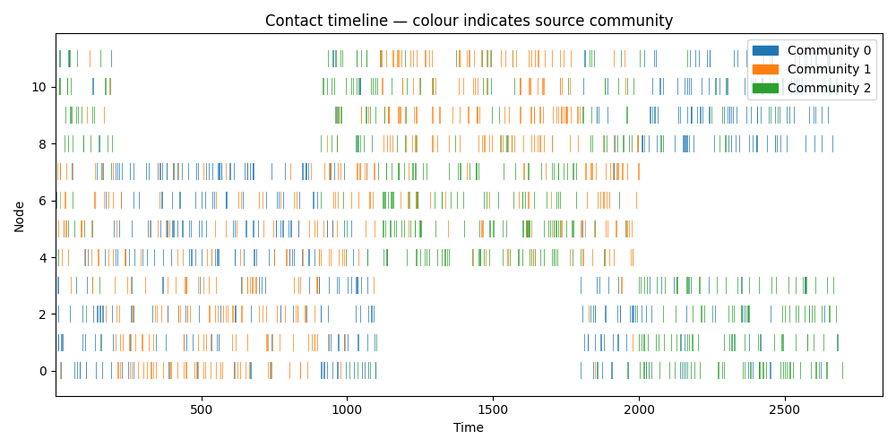
1. Contact timeline — each contact is drawn as a horizontal bar coloured by community membership of the source node.

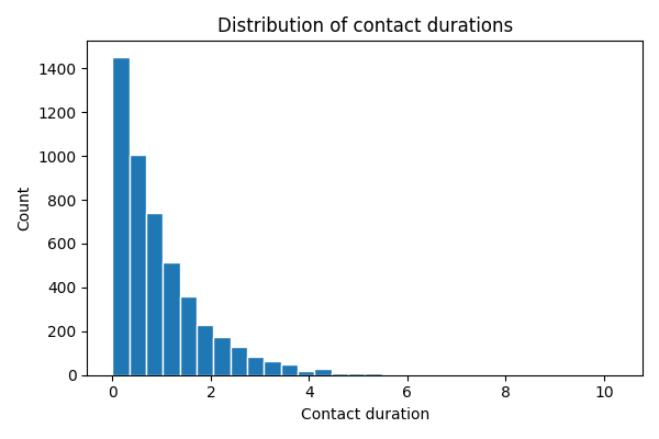
2. Event-duration distribution — histogram of all contact durations.

Setup

Create 12 Individual agents split into three equal communities (groups 0, 1, 2). Interaction durations are drawn from an exponential distribution with mean inter_tau; inter-activation waiting times use mean activ_tau.

import matplotlib.pyplot as plt
import numpy as np

from tempnet import ContTempNetwork
from tempnet.synth_temp_network import Individual, SynthTempNetwork, make_step_block_probs

rng = np.random.default_rng(42)

N_GROUPS = 3
N_PER_GROUP = 4
inter_tau = 1.0   # mean contact duration
activ_tau = 5.0   # mean inter-activation time

Individual.all_IDs = []    # reset class-level state between runs
Individual.all_groups = []

individuals = [
    Individual(
        ID=g * N_PER_GROUP + i,
        inter_distro_scale=inter_tau,
        activ_distro_scale=activ_tau,
        group=g,
    )
    for g in range(N_GROUPS)
    for i in range(N_PER_GROUP)
]

Block-probability modulation

make_step_block_probs returns a time-dependent function that cycles through phases where different community pairs are highlighted.

m1 = 0.8   # within-community interaction probability
p1 = 0.8   # cross-community interaction probability (for the active pair)

block_prob_mod_func = make_step_block_probs(
    deltat1=40 * activ_tau,
    deltat2=(9 / 2 * m1 - 3 / 2) * 40 * activ_tau / (2 * p1 - 1),
    m1=m1,
    p1=p1,
)
t_end = 3 * (40 * activ_tau + (9 / 2 * m1 - 3 / 2) * 40 * activ_tau / (2 * p1 - 1))

Run the simulation

sim = SynthTempNetwork(
    individuals=individuals,
    t_start=0,
    t_end=t_end,
    next_event_method='block_probs_mod',
    block_prob_mod_func=block_prob_mod_func,
)
sim.run()

print(
    f"Simulation produced {len(sim.indiv_sources)} contact events "
    f"over t ∈ [0, {t_end:.1f}]."
)

Warning: t must be >=0 and <= 3*(deltat1+deltat2), t is 2700.2032673748267
Simulation produced 4899 contact events over t ∈ [0, 2700.0].

Build a ContTempNetwork

network = ContTempNetwork(
    source_nodes=sim.indiv_sources,
    target_nodes=sim.indiv_targets,
    starting_times=sim.start_times,
    ending_times=sim.end_times,
)

print(f"Nodes : {network.nodes}")
print(f"Events: {len(network.events_table)}")

Nodes : [0, 1, 2, 3, 4, 5, 6, 7, 8, 9, 10, 11]
Events: 4899

Plot 1: Contact timeline

Each row is a node; each bar represents a contact coloured by the source node’s community.

GROUP_COLORS = ['#1f77b4', '#ff7f0e', '#2ca02c']  # one colour per group
node_to_group = {
    g * N_PER_GROUP + i: g
    for g in range(N_GROUPS)
    for i in range(N_PER_GROUP)
}

fig, ax = plt.subplots(figsize=(10, 5))

et = network.events_table
for _, row in et.iterrows():
    src = int(row[ContTempNetwork._SOURCES])
    tgt = int(row[ContTempNetwork._TARGETS])
    t0 = row[ContTempNetwork._STARTS]
    t1 = row[ContTempNetwork._ENDINGS]
    color = GROUP_COLORS[node_to_group[src]]
    ax.barh(tgt, t1 - t0, left=t0, height=0.6, color=color, alpha=0.7)

ax.set_xlabel('Time')
ax.set_ylabel('Node')
ax.set_title('Contact timeline — colour indicates source community')

handles = [
    plt.Rectangle((0, 0), 1, 1, color=GROUP_COLORS[g], label=f'Community {g}')
    for g in range(N_GROUPS)
]
ax.legend(handles=handles, loc='upper right')
plt.tight_layout()
plt.show()

Plot 2: Event-duration distribution

durations = (
    et[ContTempNetwork._ENDINGS] - et[ContTempNetwork._STARTS]
).values

fig, ax = plt.subplots(figsize=(6, 4))
ax.hist(durations, bins=30, edgecolor='white')
ax.set_xlabel('Contact duration')
ax.set_ylabel('Count')
ax.set_title('Distribution of contact durations')
plt.tight_layout()
plt.show()