Toy Temporal Network

This example introduces the core temporal-network workflow in tempnet. A temporal network is a graph whose edges are active only during specific time intervals: two nodes are connected for a finite period, then disconnect. Each connection is a tuple (u, v, t_start, t_end).

We build a small toy network, aggregate it into a static graph, compute the sequence of random-walk Laplacians, and finally simulate a continuous-time random walk by exponentiating those Laplacians.

import numpy as np
from matplotlib import pyplot as plt
import seaborn as sns
import tempnet as tn
import networkx as nx
from functools import reduce

Building the temporal network

Consider a small toy network with four edges:

Edge	Nodes	Active interval
1	0, 1	[0, 3]
2	1, 2	[1, 2]
3	0, 2	[2, 4]
4	1, 2	[3, 4]

To construct the temporal network, define four parallel lists – one each for source nodes, target nodes, start times, and end times – then pass them to the constructor. Each index across the four lists corresponds to a single edge.

source_nodes = [0, 1, 0, 1]
target_nodes = [1, 2, 2, 2]
starting_times = [0, 1, 2, 3]
ending_times = [3, 2, 4, 4]

tempo = tn.ContTempNetwork(
    source_nodes=source_nodes,
    target_nodes=target_nodes,
    starting_times=starting_times,
    ending_times=ending_times,
)

We can print the object to see the number of nodes and events, or access them through properties.

print(tempo)
print("num_nodes, num_events:", tempo.num_nodes, tempo.num_events)

<class 'tempnet.temporal_network.ContTempNetwork'> with 3 nodes and 4 events
num_nodes, num_events: 3 4

The full cleaned dataframe is available in one go, including a durations column derived from the start and end times.

print(tempo.events_table)

   source_nodes  target_nodes  starting_times  ending_times  durations
0             0             1               0             3          3
1             1             2               1             2          1
2             0             2               2             4          2
3             1             2               3             4          1

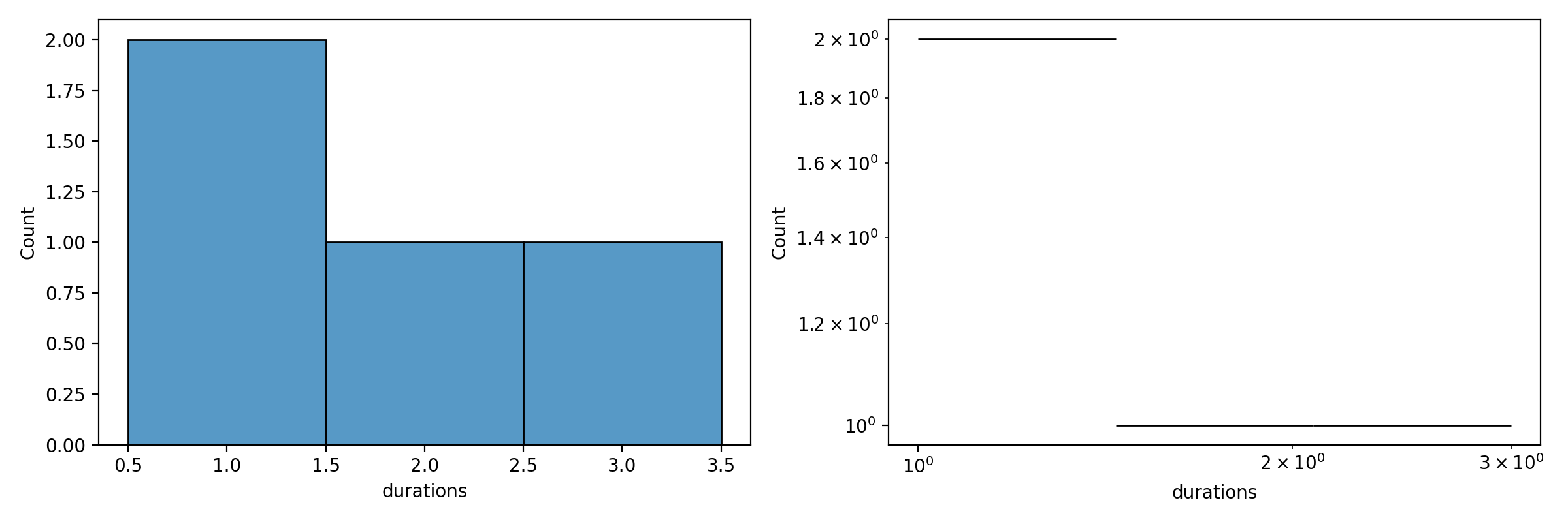
Distribution of edge activation durations

The durations column lets us inspect the distribution of edge activation periods, shown here in both linear and log scale.

fig, ax = plt.subplots(nrows=1, ncols=2, figsize=(12, 4), dpi=200)
sns.histplot(data=tempo.events_table, x="durations", ax=ax[0], discrete=True)
sns.histplot(data=tempo.events_table, x="durations", ax=ax[1], log_scale=(True, True))
plt.tight_layout()
plt.show()

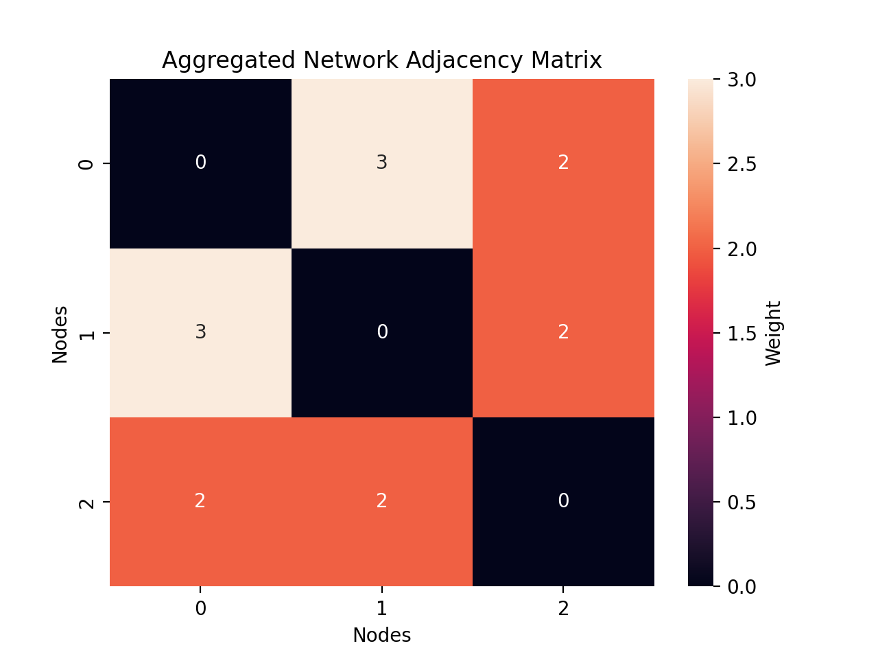
Aggregating into a static network

We can collapse the time dimension entirely, aggregating the temporal network into a static graph. This is visualized as a heatmap, where each cell’s color represents the total weight of edge activations between a pair of nodes.

A = tempo.compute_static_adjacency_matrix()

fig, ax = plt.subplots(nrows=1, ncols=1, dpi=200)
sns.heatmap(A.toarray(), ax=ax, annot=True, cbar_kws={"label": "Weight"})
ax.set_xlabel("Nodes")
ax.set_ylabel("Nodes")
ax.set_title("Aggregated Network Adjacency Matrix")
plt.show()

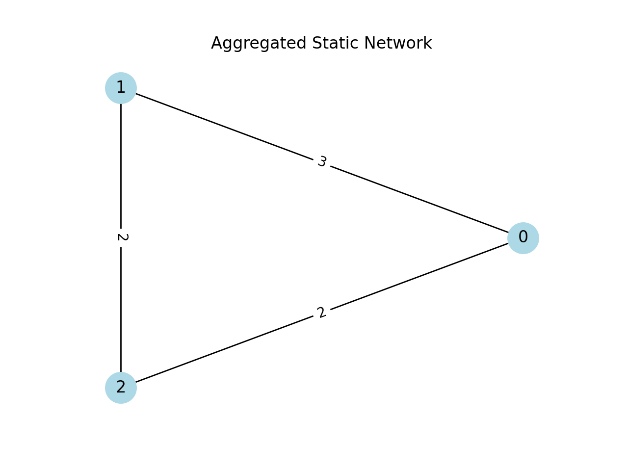
We then transform it into a NetworkX object to visualise and run other algorithms on it.

static = nx.from_numpy_array(A.toarray())

pos = nx.circular_layout(static)

fig, ax = plt.subplots(nrows=1, ncols=1, dpi=200)
nx.draw(static, pos, with_labels=True, node_color="lightblue", node_size=500)
edge_labels = nx.get_edge_attributes(static, "weight")
nx.draw_networkx_edge_labels(static, pos, edge_labels=edge_labels)
plt.title("Aggregated Static Network")
plt.show()

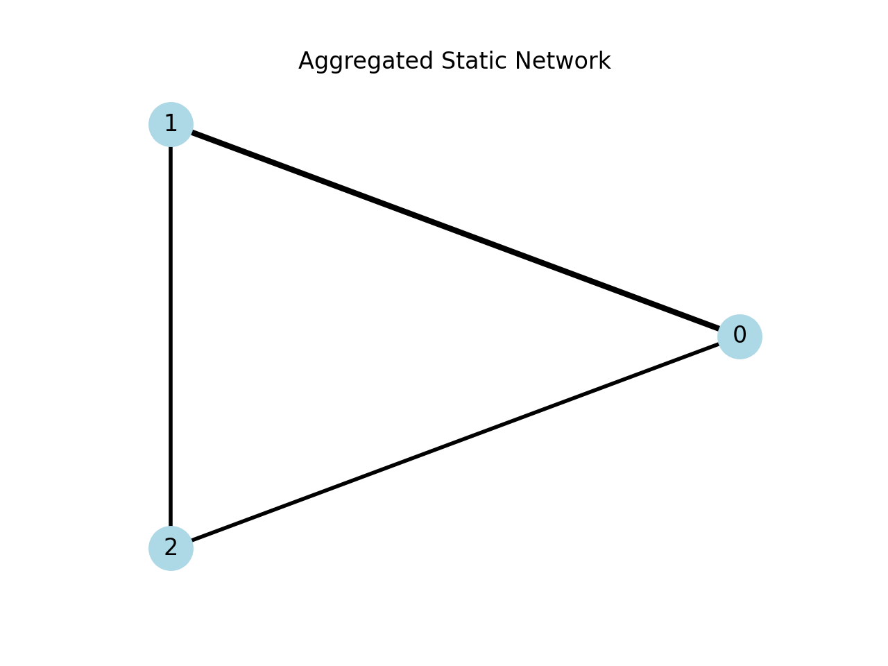
Alternatively, we can represent edge weights as the thickness of each edge.

fig, ax = plt.subplots(nrows=1, ncols=1, dpi=200)

weights = [static[u][v]["weight"] for u, v in static.edges()]
max_w = max(weights)
widths = [3 * w / max_w for w in weights]

nx.draw(
    static,
    pos,
    with_labels=True,
    width=widths,
    node_color="lightblue",
    node_size=500,
)
plt.title("Aggregated Static Network")
plt.show()

Inspecting nodes and timestamps

Back in the temporal representation, we can access the list of nodes, all timestamps, and the start/end of the network (the minimum start time and maximum end time).

tempo._compute_time_grid()
print("Node array", tempo.node_array)
print("Timestamps", tempo.times)
print("Start:", tempo.start_time)
print("End:", tempo.end_time)

Node array [0 1 2]
Timestamps Index([0, 1, 2, 3, 4], dtype='int64', name='times')
Start: 0
End: 4

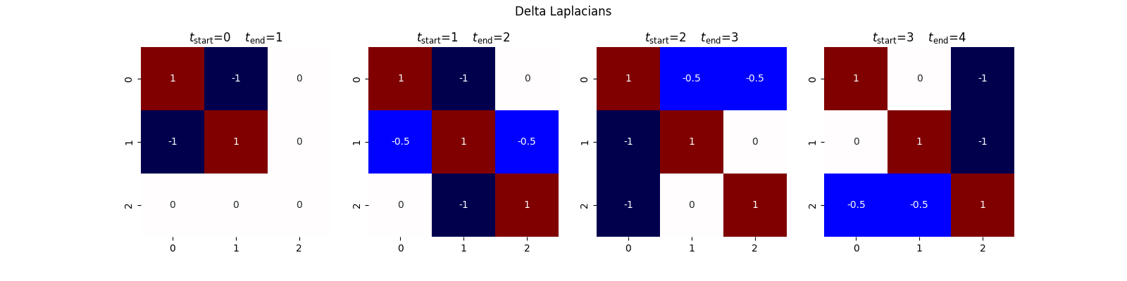
Random-walk Laplacians

This package implements the continuous-time random walk on temporal networks, which can be used to capture conditional entropy, assortativity, and community detection via flow stability.

Given a temporal network with ordered timestamps \(t_0, t_1, \dots, t_T\), we construct a sequence of graph snapshots. For each consecutive pair \((t_i, t_{i+1})\), we extract the subgraph of edges active during that interval and compute its random walk Laplacian.

For a snapshot with adjacency matrix \(A\) and degree matrix \(D = \mathrm{diag}(d_1, \dots, d_n)\), the random walk Laplacian is

\[L_{\mathrm{rw}} = I - D^{-1}A\]

where \(I\) is the identity matrix. If a node \(i\) has degree \(d_i = 0\) in a given snapshot, \(D^{-1}\) is undefined; to handle this, we make the random walker stay in place by adding a self-loop (\(A_{ii} = 1\), \(d_i = 1\)). This yields one Laplacian per interval \([t_i, t_{i+1})\).

tempo.compute_laplacian_matrices()

We can directly access the delta Laplacian matrices for inspection.

fig, ax = plt.subplots(nrows=1, ncols=4, figsize=(16, 4))
for i in range(4):
    sns.heatmap(
        tempo.laplacians[i].toarray(),
        ax=ax[i],
        square=True,
        annot=True,
        cbar=False,
        vmin=-1,
        vmax=1,
        cmap="seismic",
    )
    ax[i].set_title(
        rf"$t_{{\text{{start}}}}$={tempo.times[i]}"
        "\t"
        rf"$t_{{\text{{end}}}}$={tempo.times[i + 1]}"
    )
fig.suptitle("Delta Laplacians")
plt.show()

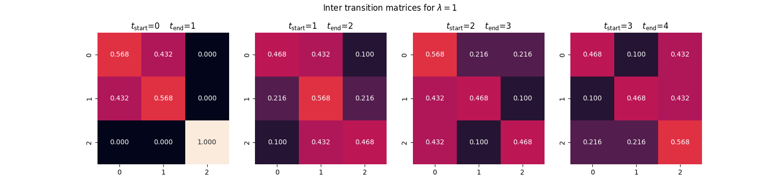
Transition matrices

With the random-walk Laplacians computed, we simulate the continuous-time random walk by computing the matrix exponential of each Laplacian, scaled by the duration of the corresponding interval and the walker’s transition rate. For two consecutive timestamps \(t_i\) and \(t_{i+1}\),

\[T_{\lambda_{\mathrm{RW}}}^{(i)} = \exp\!\left(-\lambda_{\mathrm{RW}}\, \Delta t\, L_{\mathrm{rw}}^{(i)}\right)\]

where \(\Delta t = t_{i+1} - t_i\) and \(\lambda_{\mathrm{RW}}\) is the rate of the random walker. The entry \(T_{jk}^{(i)}\) gives the probability that a walker starting at node \(j\) at time \(t_i\) reaches node \(k\) at time \(t_{i+1}\).

tempo.compute_inter_transition_matrices(lamda=1)
inter_transition_matrices = tempo.inter_T[1]

fig, ax = plt.subplots(nrows=1, ncols=4, figsize=(16, 4))
for i in range(4):
    sns.heatmap(
        inter_transition_matrices[i].toarray(),
        ax=ax[i],
        square=True,
        annot=True,
        cbar=False,
        fmt=".3f",
        vmin=0,
        vmax=1,
    )
    ax[i].set_title(
        rf"$t_{{\text{{start}}}}$={tempo.times[i]}"
        "\t"
        rf"$t_{{\text{{end}}}}$={tempo.times[i + 1]}"
    )
fig.suptitle(r"Inter transition matrices for $\lambda=1$")
plt.show()

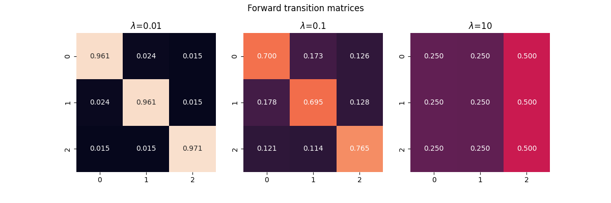
Forward transition matrix

The forward transition matrix is the product of the inter-transition matrices:

\[T_{\lambda_{\mathrm{RW}}} = \prod_{i=0}^{T-1} T_{\lambda_{\mathrm{RW}}}^{(i)}\]

The entry \(T_{jk}\) gives the probability that a walker with rate \(\lambda_{\mathrm{RW}}\), starting at node \(j\) at the beginning of the network, arrives at node \(k\) by the end. The rate controls the walker’s exploration speed:

• Low rate (\(\lambda_{\mathrm{RW}} \ll 1\)): the walker barely moves, so \(T\) remains close to the identity matrix.

• High rate (\(\lambda_{\mathrm{RW}} \gg 1\)): the walker mixes rapidly, washing out temporal structure.

fig, ax = plt.subplots(nrows=1, ncols=3, figsize=(12, 4))
for i, lamda in enumerate([1e-2, 0.1, 10]):
    tempo.compute_inter_transition_matrices(lamda=lamda)
    matrix = reduce(lambda a, b: a @ b, tempo.inter_T[lamda])
    sns.heatmap(
        matrix.toarray(),
        ax=ax[i],
        square=True,
        annot=True,
        cbar=False,
        fmt=".3f",
        vmin=0,
        vmax=1,
    )
    ax[i].set_title(rf"$\lambda$={lamda}")
fig.suptitle("Forward transition matrices")
plt.show()