Mouse contact network (empirical data)

This example loads the mouse proximity-contact dataset published by König (2021) and analyses it as a continuous-time temporal network using ContTempNetwork.

The dataset records pairwise contact events (start time, end time, source mouse, target mouse) collected over several days.

The example walks through the duration distribution, the aggregated static adjacency matrix and network, node and event activity over time, the raw contact timeline. and finally the forward transition matrices at several time scales.

Load libraries

import tempfile
from functools import reduce
from pathlib import Path

import numpy as np
import pandas as pd
import networkx as nx
import seaborn as sns
from matplotlib import pyplot as plt
from matplotlib.colors import LogNorm

from zenodo_get import download

import tempnet as tn

Download and load the dataset

We fetch the contact sequence from Zenodo and directly convert it to a DataFrame.

RECORD_ID = "4725155"
FILE_NAME = "mice_contact_sequence.csv.gz"

with tempfile.TemporaryDirectory() as tmpdir:
    download(
        record_or_doi=RECORD_ID,
        output_dir=tmpdir,
        file_glob=FILE_NAME,
    )
    event_table = pd.read_csv(Path(tmpdir) / FILE_NAME, compression="gzip")

2026-06-16 12:03:17.324 | INFO     | zenodo_get.zget:_zenodo_download_logic:328 - Output directory: /tmp/tmp6z78j4p1
2026-06-16 12:03:17.842 | INFO     | zenodo_get.zget:_zenodo_download_logic:426 - Title: Temporal contact network of a free-ranging house mice population
2026-06-16 12:03:17.842 | INFO     | zenodo_get.zget:_zenodo_download_logic:438 - Total size: 53.7 MB
2026-06-16 12:03:17.842 | INFO     | zenodo_get.zget:_zenodo_download_logic:439 - Number of files: 1

Files:   0%|          | 0/1 [00:00<?, ?file/s]
Files: 100%|██████████| 1/1 [00:16<00:00, 16.40s/file]

2026-06-16 12:03:34.253 | SUCCESS  | zenodo_get.zget:_zenodo_download_logic:487 - All specified files have been processed.

Filter the events

We round the times, and keep only the first day of activity.

event_table = event_table.round(2)

# filter 1 hour
event_table = event_table[event_table['ending_times'] <= 24*3600].reset_index(
    drop=True
)

Inspect the first few rows of the event table.

print(event_table.head())

   source_nodes  target_nodes  starting_times  ending_times  durations
0            61            67           11.13         37.85      26.73
1           270           276           12.68        137.17     124.49
2           256           269           12.82         64.95      52.13
3           256           398           20.90         49.94      29.04
4           269           398           20.90         49.94      29.04

Build the continuous-time temporal network

tempo = tn.ContTempNetwork(events_table=event_table)

Now we find the number of nodes and number of events.

print(tempo)

<class 'tempnet.temporal_network.ContTempNetwork'> with 414 nodes and 132034 events

We can also access the variables directly from the object:

print('Number of mice', tempo.num_nodes)
print('Number of events', tempo.num_events)

Number of mice 414
Number of events 132034

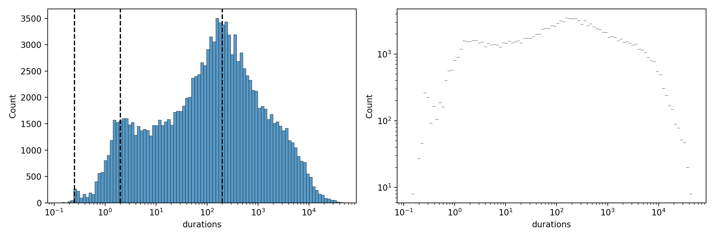
Event-duration distribution

Histogram of contact durations on log-linear and log-log axes.

fig, ax = plt.subplots(nrows=1, ncols=2, figsize=(12, 4), dpi=200)
sns.histplot(data=tempo.events_table, x='durations', ax=ax[0],
             log_scale=(True, False))
sns.histplot(data=tempo.events_table, x='durations', ax=ax[1],
             log_scale=(True, True))
ax[0].axvline(0.25, color='k', linestyle='--')
ax[0].axvline(2, color='k', linestyle='--')
ax[0].axvline(200, color='k', linestyle='--')

plt.tight_layout()
plt.show()

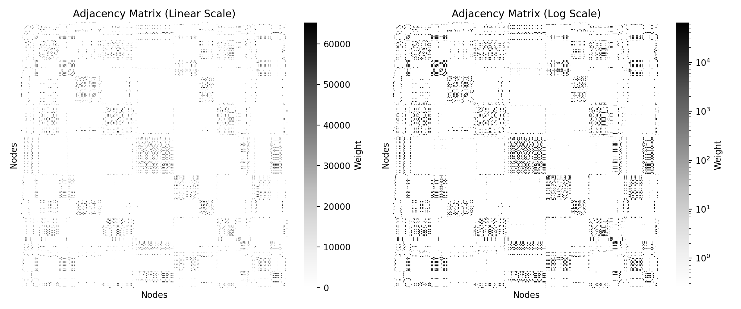
Static aggregated adjacency matrix

We aggregate the temporal network into a static weighted adjacency matrix and display it on linear and logarithmic colour scales.

A = tempo.compute_static_adjacency_matrix()
A_dense = A.toarray()

fig, (ax1, ax2) = plt.subplots(nrows=1, ncols=2, dpi=200, figsize=(12, 5))

sns.heatmap(A_dense, ax=ax1, cbar_kws={'label': 'Weight'}, cmap='Greys')
ax1.set_xlabel('Nodes')
ax1.set_ylabel('Nodes')
ax1.set_xticks([])
ax1.set_yticks([])
ax1.set_title('Adjacency Matrix (Linear Scale)')

A_log = A_dense.copy()
A_log[A_log == 0] = np.nan

sns.heatmap(A_log, ax=ax2, norm=LogNorm(), cbar_kws={'label': 'Weight'},
            cmap='Greys')
ax2.set_xlabel('Nodes')
ax2.set_ylabel('Nodes')
ax2.set_xticks([])
ax2.set_yticks([])
ax2.set_title('Adjacency Matrix (Log Scale)')

plt.tight_layout()
plt.show()

Convert to a NetworkX graph

We then transform it into a NetworkX object to visualise and perform other algorithms and measure computation.

static = nx.from_numpy_array(A.toarray())

Check whether the aggregated network is connected.

print(nx.is_connected(static))

False

Draw the aggregated static network, with edge widths scaled by weight.

fig, ax = plt.subplots(nrows=1, ncols=1, dpi=200)

pos = nx.spring_layout(static, seed=412)
weights = [static[u][v]["weight"] for u, v in static.edges()]
max_w = max(weights)
widths = [2 * np.log10(w) / np.log10(max_w) for w in weights]

nx.draw(static, pos, with_labels=False, width=widths, node_color="teal",
        node_size=5)

plt.title("Aggregated Static Network")
plt.show()

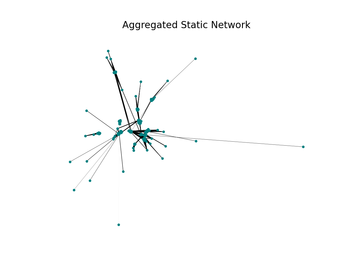
The network is not connected, and it is clearly modular.

To find the start and end of the temporal network – equivalently, the minimum start time and maximum end time – we can query the network directly:

print("Start:", tempo.start_time)
print("End:", tempo.end_time)

Start: 11.13
End: 86391.0

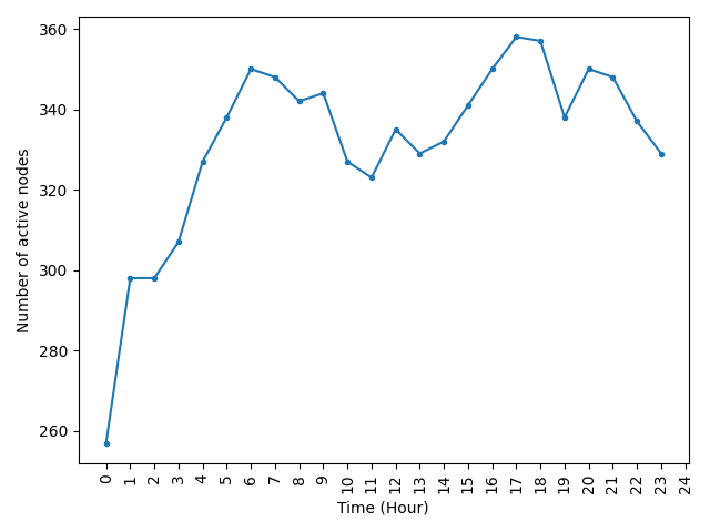
Active nodes over time

Number of active nodes in each one-hour window across a full day.

t = np.arange(0, 24 * 3600 + 1, 3600)
n_active = [tempo.num_active_nodes(t[i], t[i + 1]) for i in range(len(t) - 1)]
fig, ax = plt.subplots(nrows=1, ncols=1)
ax.plot(t[:-1], n_active, marker='.')

ax.set_xticks(t)
ax.set_xticklabels([i // 3600 for i in t], rotation=90)
ax.set_xlabel('Time (Hour)')
ax.set_ylabel('Number of active nodes')
plt.tight_layout()
plt.show()

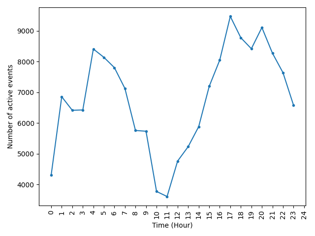
Active events over time

Number of active edges/events in each one-hour window.

t = np.arange(0, 24 * 3600 + 1, 3600)
n_edge_active = [tempo.num_active_edges(t[i], t[i + 1])
                 for i in range(len(t) - 1)]

fig, ax = plt.subplots(nrows=1, ncols=1)
ax.plot(t[:-1], n_edge_active, marker='.')

ax.set_xticks(t)
ax.set_xticklabels([i // 3600 for i in t], rotation=90)
ax.set_xlabel('Time (Hour)')
ax.set_ylabel('Number of active events')
plt.tight_layout()
plt.show()

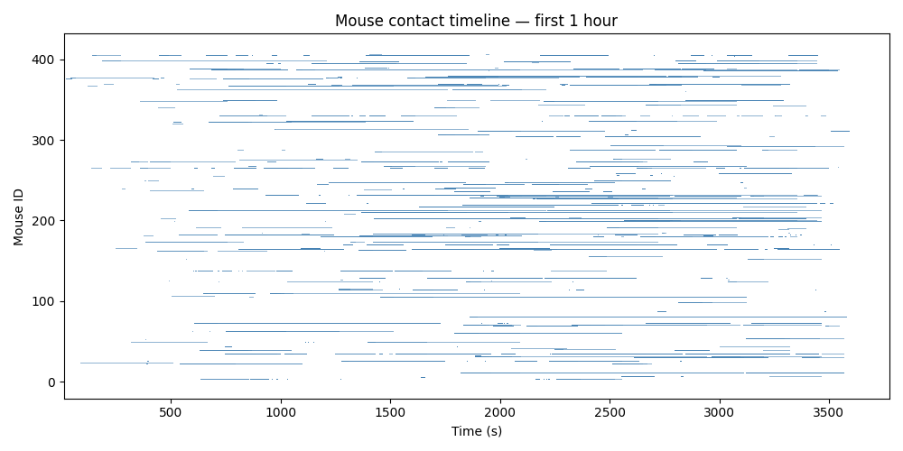
Mouse contact timeline

The activity of events and nodes depends on the time of day. We can also investigate the network in the first hour. Each contact is drawn as a horizontal bar; rows correspond to individual mice.

fig, ax = plt.subplots(figsize=(10, 5))
et = tempo.events_table
et = et[et['ending_times'] <= 3600]

for _, row in et.iterrows():
    tgt = row[tempo._TARGETS]
    t0 = row[tempo._STARTS]
    t1 = row[tempo._ENDINGS]
    ax.barh(tgt, t1 - t0, left=t0, height=0.6, color='steelblue', alpha=0.6)

ax.set_xlabel('Time (s)')
ax.set_ylabel('Mouse ID')
ax.set_title('Mouse contact timeline — first 1 hour')
plt.tight_layout()
plt.show()

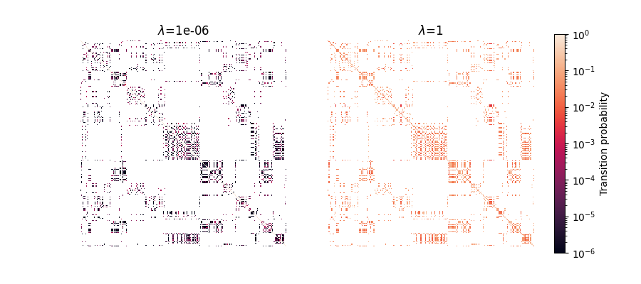
Forward transition matrices

Now we want to compute the forward transition matrices by first computing the Laplacians for the 1st hour to keep the example fast enough.

tempo = tn.ContTempNetwork(events_table=et)
tempo.compute_laplacian_matrices()

We then proceed to computing the forward transition matrix for 3 time scales. It may take few minutes to run this.

scales = [1e-6, 1]
for i, s in enumerate(scales):
    tempo.compute_inter_transition_matrices(lamda=s)

forward_transition_matrices = [
    reduce(lambda a, b: a @ b, tempo.inter_T[s]) for s in scales
]

Visualise the forward transition matrices for each time scale.

norm = LogNorm(vmin=1e-6, vmax=1)
fig, ax = plt.subplots(nrows=1, ncols=2, figsize=(9, 4))
for i, (lamda, matrix) in enumerate(zip(scales, forward_transition_matrices)):
    sns.heatmap(matrix.toarray(), ax=ax[i], square=True, cbar=False,
                norm=norm)
    ax[i].set_title(rf'$\lambda$={lamda}')
    ax[i].set_xticks([])
    ax[i].set_yticks([])

fig.colorbar(ax[0].collections[0], ax=ax, label='Transition probability',
             fraction=0.046, pad=0.04)
plt.show()